This is the second chapter of the DB engineering series. As a prerequisite ensure that you read the first chapter about databases storing the data here.
Jump to other chapters:
- 01. Understanding database storage
- 02. Database Indexes
- 03. Understanding EXPLAIN & ANALYZE
- 04. Partitioning
- 05. Sharding
- 06. Transactional vs Analytical Databases
Creating a table with a million rows
Before we move forward about learning indexes, let’s first create a table and populate the same with data. First, let’s create a people table with 3 attributes.
CREATE TABLE people (
  id serial PRIMARY KEY,
  name text,
  age int,
  salary int
);
Let’s insert 1M records into the table
INSERT INTO people (name, age, salary)
SELECT
substring('ABCDEFGHIJKLMNOPQRSTUVWXYZabcdefghijklmnopqrstuvwxyz0123456789', (random() * 62 + 1)::int, 5),
random() * 100 + 18,
random() * 100000 + 10000
FROM generate_series(1, 1000000);
Now we have enough records to try querying.
learning_test=> SELECT count(*) FROM people;
  count
---------
 1000000
(1 row)
All of us have our contacts saved on our phones. In the olden days, there were phonebooks that organized the names and numbers. In a phonebook, the numbers are sorted by name. This makes it easy to find someone’s phone number by their name. If the phonebook were just a list of names and numbers, it would be much more difficult to find someone’s phone number.
Database indexes work in the same way. They store information about the data in a more organized way, which makes it easier to find the data you’re looking for. Database indexes can be used to speed up all sorts of queries, including searches, sorts, and joins. They are an essential part of any database system.
Let’s describe the table which we created.
learning_test=> \d people;
                            Table "public.people"
 Column |  Type   | Collation | Nullable |              Default
--------+---------+-----------+----------+------------------------------------
 id     | integer |           | not null | nextval('people_id_seq'::regclass)
 name   | text    |           |          |
 age    | integer |           |          |
 salary | integer |           |          |
Indexes:
    "people_pkey" PRIMARY KEY, btree (id)
In the above output, we can see that the primary key id has an index people_pkey. There are no other indexes for the table.
Let’s try to query all the people who are at 40 years of age.
SELECT * FROM people where age = 40;The output for the above query is fairly large. Let’s check the query plan for the above. We will learn more about understanding EXPLAIN and ANALYZE in the next chapter. Simply put
EXPLAINgives us a review the execution plan of the query. Coupling withANALYZE, will give us the execution timings of the query.
learning_test=> EXPLAIN ANALYZE SELECT * FROM people WHERE age = 40;
                                             QUERY PLAN
---------------------------------------------------------------------------------------------------------------------------
 Gather  (cost=1000.00..13484.03 rows=9467 width=17) (actual time=0.271..95.911 rows=10176 loops=1)
   Workers Planned: 2
   Workers Launched: 2
   ->  Parallel Seq Scan on people  (cost=0.00..11537.33 rows=3945 width=17) (actual time=0.018..80.237 rows=3392 loops=3)
         Filter: (age = 40)
         Rows Removed by Filter: 329941
 Planning Time: 0.158 ms
 Execution Time: 96.414 ms
(8 rows)
The key points to note from the above plan are that
- The DB scanned all the rows (Seq Scan) for rows matching the condition (age = 40).
- It took ~96ms to complete the query.
Now let’s add an index based on age to the table.
CREATE INDEX idx_age_people ON people(age); Now let’s rerun the query plan again.
                                                           QUERY PLAN
--------------------------------------------------------------------------------------------------------------------------------
 Bitmap Heap Scan on people  (cost=109.79..6861.53 rows=9467 width=17) (actual time=1.441..8.195 rows=10176 loops=1)
   Recheck Cond: (age = 40)
   Heap Blocks: exact=5045
   ->  Bitmap Index Scan on idx_age_people  (cost=0.00..107.43 rows=9467 width=0) (actual time=0.648..0.649 rows=10176 loops=1)
         Index Cond: (age = 40)
 Planning Time: 0.191 ms
 Execution Time: 8.738 ms
(7 rows)
Tada!
The execution has dropped to ~9ms (an approx 11x drop).
Now if we describe the table, we can see that there is a new index added.
learning_test=> \d people;
                            Table "public.people"
 Column |  Type   | Collation | Nullable |              Default
--------+---------+-----------+----------+------------------------------------
 id     | integer |           | not null | nextval('people_id_seq'::regclass)
 name   | text    |           |          |
 age    | integer |           |          |
 salary | integer |           |          |
Indexes:
    "people_pkey" PRIMARY KEY, btree (id)
    "idx_age_people" btree (age)
When the database queries the rows, at a very high level, the following is what happens.
- The DB will check the age index first.
- It then picks up all the row_ids that match the age = 40.
- Once the DB knows the rows, instead of scanning the full table, the DB goes to relevant pages of the heap where these rows are present and picks those alone.
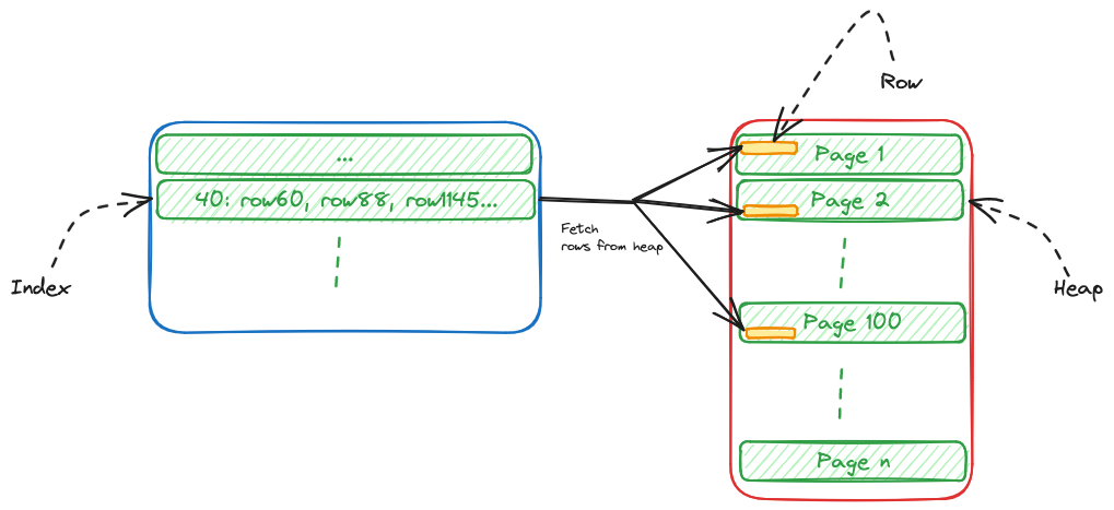
The above process is significantly faster than scanning the full table for rows that match age = 40.
Types of indexes
From the output of the table description, you can see that both indexes are of the type btree. btree indexes are very commonly used in databases. B-tree is a sorted tree data structure that allows insertions, deletions, and searching in logarithmic time [O(log(n))]. B-tree indexes work great for comparisons.
Other indexes worth mentioning are
- Hash indexes
Hash indexes can be used for equality comparison. Hash indexes store a hash value of the indexed column, which can be used to quickly find rows that match a specific value. Unlike B-tree indexes, hash indexes are not good for range queries. - GiST indexes
GiST (Generalized Search Tree) indexes are used for full-text searches and geometric data types. GiST indexes are more efficient for queries that use range operators, such as “greater than” and “less than.” - GIN indexes
GIN indexes are a type of inverted index that is optimized for storing and querying composite values. - BRIN indexes
BRIN (Block Range Index) is a type of index that is designed for large tables, for range queries and is used frequently.
Choosing the right index type and columns to index depends on the type of queries your application will fire. Indexes will improve the read performance of queries especially queries that are highly selective.
DB Indexes Quiz
Next, we will see how to check in more detail whether your indexes are actually getting used with EXPLAIN and ANALYZE.
Read here.